Glowing lines in QGIS

In one of my previous QGIS posts, on flow mapping, I outlined a method for mapping origin-destination data related to movements, rendered as a collection of straight lines from point a to b. One thing I didn't do in that post was explain how you get the 'glow' effect to make the lines appear brighter at higher densities (example below).

A little glowing flow map example from my US commuting map

Since a few people have asked about it, I thought I'd share it - and thanks to Nyall Dawson and all the other QGIS developers for making this possible. If I begin with a commuting flow dataset I made for England and Wales and just add it to QGIS, here's what I get (click on the individual images to see them full size):

We can see the country outline, that's about it

Next, let's try reducing the default line width from 0.26 to 0.1 and see what happens...

This is a bit clearer, but still not very useful.

We could darken the background (via Project > Project Properties > General) to make the lines stand out more...

This is getting a bit better now, but still not great

Okay, let's now change the colour and introduce some feature transparency and see how this looks:

Definitely an improvement, but not great

Note how this was done, if you don't already know:

So far, so good. But what about the glow effects? That's where feature blending mode comes in - as you can see below:

With a line width of 0.1, transparency of 90% (because I have a couple of million lines here) and a Feature blending mode set to 'Addition' here's what I get:

You may need a different transparency % in your data

What on earth do all the different blending modes do? There's 'Screen', 'Multiply', 'Dodge' and many more but it's not immediately obvious so here's a little summary from the QGIS 2.8 documentation pages on the subject:

To see the different impact each feature blending mode has, it's best to try them - for example, if you want a less 'glowy' version of the previous example above, you could used 'Dodge', as shown below:

Similar to the previous one, but this is 'Dodge'

Of course, you could also decide that you want the lines to be different colours and symbolise them differently based on their length. With this, you take a different approach and it would look something like the image below, where I've used reds:

No feature blending here, just layer symbology and ordering

To achieve the above, you'd have to have a line length field (but that's easy in QGIS) and then color different lengths slightly differently and then use layer ordering. This too requires a good bit of experimenting to get right (and the ones shown here are far from perfect examples) but here's an example from the layer properties dialogue:

Note: click 'Advanced' to see symbol levels

The only other thing to mention is that when you zoom in you'll see things differently and perhaps need to change the symbology to suit the zoom level. You can see this for the example below where I've zoomed in to London and changed the transparency down to 70%:

Now we can begin to make more sense of the flows

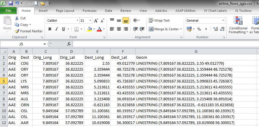
If you want to know how to create the flow lines in the first place, check out my previous post on the subject, where I also provide a sample dataset to work with. Once you've got things looking as you want them, you can then add labels and all sorts of other things to make your map more informative. Note that I used QGIS 2.10 here but this should work from QGIS 2.2 and above.

Mapping the American Commute

Update, 20 September 2015: scroll to the bottom of the post if you want to download the data.

One of my summer projects this year has been attempting to map the American commute, following earlier work on a similar subject. Put simply, I've attempted to put together a map which shows commuting connections between locations in the contiguous United States, using the most fine-grained data I could find. Some of the results of this went into a recent piece in WIRED, and also CityMetric, and the larger piece of work it's based on is part of on-going research into the best ways of mapping commuting flows. The main images are below, followed by some more technical information. For now, all you need to know is that these images show commuting connections of 100 miles or less between Census tracts in the lower 48 states. You'll have to forgive me if your city isn't labelled! 

Higher resolution image available here

And now some zoomed in versions...

Zoom in of the west coast

Texas, and beyond!

Interesting patterns of connectivity in the Midwest

Look closely for some interesting inter-connections

The famous BosWash megalopolis

But this just shows where people live, doesn't it? Yes it does. But it also shows how the places where people live connect with other places from a functional economic point of view, at a fairly fine-grained level. It offers a slightly different view than just looking at the urban fabric alone which, I might add, is interesting in itself. Mapping flows like this is not exactly new, as this paper from Arthur Robinson (1955) on Henry Drury Harness (1837) demonstrates. Nonetheless, I haven't seen anyone map travel to work at this resolution for the United States, so I thought I'd have a go myself. 

If you spend some time looking at the big version of the map you can begin to see how places connect and where there are obvious disconnections, even between places that are not that far apart. One thing that you can pick up from the complete dataset (but not this batch of maps) is the growth of mega-commuting, as explained by Melanie Rapino and Alison Fields of the United States Census Bureau. 

Background information: the data I used is the most recent tract-to-tract journey to work dataset from the American Community Survey. This dataset covers journeys to work between the c74,000 census tracts in the United States and the complete dataset has around 4million interactions. I mapped this in QGIS, using methods I've described previously on this blog. The tricky bits were dealing with the messy FIPS codes, dealing with the size of the dataset, and trying to decide what to label. There is quite a bit of error in the dataset (as acknowledged by the ACS people) and each individual flow line has a margin of error value associated with it, from which I also calculated the coefficient of variation. This is explained in a more detailed working paper, which I expect to publish in the coming months.

Update, 20 September 2015: there has been quite a bit of interest in the underlying dataset I put together to create the maps, so I have decided to make the whole shapefile available here in the hope that others will find it useful and be able to produce some interesting analysis or visuals from it. I'm hoping someone will do a cool interactive web map of it, but it might be quite technically challenging. If you do use it, make sure you read the associated working paper, which explains the process and the underlying data. One word of warning: the uncompressed file is pretty big so you'll need a good computer.

Mapping the American Commute: download the data (213MB, zipped shapefile)

Visualising Residential Mobility in Urban England

Last year I produced a few commuting maps of England and Wales after the 2011 Census data were released. Now I've turned my attention to mapping patterns of residential mobility in urban areas of England as part of my work on understanding housing markets. This post highlights some of the patterns uncovered in the data - which are output area level migration flows for England and Wales (about 4 million individual flows). If you're interested in how I did this you can find out in a previous post. The first image is of the urban North West of England and for subsequent images I've zoomed to different parts of the country. I've kept it simple and only showed the flow lines, apart from in the North West where I've also added some place labels. It's all a bit experimental at this stage.

You can find a higher resolution image here

The North East of England

West, East and South Yorkshire

I think some places are missing (working on it)

I've adjusted the brightness a little to make this clearer

What does all this show? It shows what many people may already know or expect but basically it illustrates the extent of residential mobility patterns in some of England's major urban areas - plus a bit more in the South West example above. There's a lot more that could be said about this but for now I'll leave it at that. I'm sorry if your town or city isn't on the map! Maybe next time...

Notes: I've filtered the data so in certain cases some places are not shown (e.g. in the North West image places in North Wales are not visible). Also, I've only shown flows of a certain volume in order to filter out the noise. 

Simple Animations with QGIS - A Long Tutorial

This rather long post explains how you can make images and animations like the ones below using only open source software (mostly QGIS) and open data. I've just used flights from Hartsfield-Jackson International Airport in Atlanta because it's the busiest airport in the world and serves a wide variety of destinations. The methods are relatively straightforward but it does take time to get your head around if you're new to the software and the data. If you're already a competent QGIS user it should be pretty easy. Once you've got the method nailed down you can apply it to all kinds of different scenarios and datasets. First of all, though, here's a static image of outbound flights from ATL projected onto a globe.

Flight destinations from Atlanta (full size)

The first thing you'll need to do is get some data. In this example I've taken some general country boundaries from Natural Earth and for the flights data I've used the OpenFlights dataset. I then created an azimuthal orthographic projection centred on Hartsfield-Jackson International Airport in Atlanta. Hamish Campbell already wrote an excellent tutorial on how to do this in QGIS, so just follow that if you want to use a projection that makes your country layer appear as if it were on a globe. The only extra tips you'll perhaps need to replicate Hamish's method are as follows. To get the lat/long of a place you want to centre your projection on, just search for it on Google Maps and then look in the address bar for the coordinates. The python script on Hamish's page just needs to be copied and pasted into a text document, saved with a .py extension and then placed in the correct folder on your computer (on a PC with QGIS 2.4 it would be something like this: C:\Program Files\QGIS Chugiak\bin). Also, when you clip the layer to a global projection, QGIS will create a clip circle and a new clipped layer. These may not appear at all or if they do they'll maybe be very blocky. If so, go to the properties for the layer in QGIS and on the Rendering tab just untick 'Simplify Geometries'. I normally save new copies of these layers using Save As... from each layer.

A faster animated version of ATL outbound flights (big)

That should be your global projection sorted. You can then apply it via the Project menu in QGIS and then Project Properties... CRS and then 'Project on the fly' as in the tutorial.  To achieve some of the visual effects above, I just duplicated the clipped circle layer (you'll have to Save As... from the temp clipped layer to do this) and applied an inverted polygon style and a shapeburst fill with a blue to black gradient (Nyall Dawson did a great blog post on this, which you might find useful). I also did a similar thing with the land layer, just to make some of the smaller islands stand out. You'll also need to make the outline colour the same as the fill colour in the circle to avoid a line appearing through your earth.

A very slow version, with a pause at the end (big)

So far, so good. But what about the flight paths and animated dots? Well, to create the lines you can follow my blog post on flow mapping in QGIS and use the sample dataset I posted there. You'll need to calculate two new columns for this shapefile (see below) and use the MMQGIS plugin for QGIS (installed, as ever, via the Plugins menu). If you just add this file to your global azimuthal orthographic projection there will be so many lines and it may take a long time to display so there are a few intermediate steps I'd recommend... 

1. Open the new global flights dataset in a blank QGIS project using the default projection and then remove duplicate lines using Modify, Delete Duplicate Geometries in the MMQGIS plugin. Many routes (e.g. JFK-LHR) are served by multiple airlines and I wanted to only show origins and destinations. This also makes the file much smaller. 2. Although the flight connections would appear as straight lines on our global projection, I like them to look a little curved; partly for effect and partly to bring out the curvature of the earth but also because flight paths are not straight lines in reality. So, once I've removed duplicates I then 'densify' the lines in QGIS by adding in 50 intermediate vertices - done via Vector, Geometry Tools, Densify polygons in QGIS. 3. I then added this new flights layer to my ATL-based global projection and I clipped the layer using the Hamish Campbell method, and saving the resulting layer as a new shapefile. You should now have a globe centred on the location of your choice, plus some nice curved airline flight paths.

Same as above, but with labels and pause at end (big)

For the next stage, the way I did it was to open the dbf part of the new flight paths shapefile in Excel and then calculate an 'offset' lat and long column which I could use to animate the dots. You just need to read the Animate Columns part of Michael Minn's MMQGIS page to understand this. Once you've calculated the new lat/long offset columns you can save the csv. Once you've done this, import the csv into QGIS using the Add Delimited Text Layer (comma icon), using the airport origin lat/long as the x,y coordinates in the import dialogue. Filter the new layer so it only shows ATL origins and you'll just see one dot for ATL but actually there are many dots in the same location as they all have the same origin lat/long. Save the filtered layer as a new shapefile and then run the Animate Columns tool in MMQGIS using the appropriate fields and the number of animation frames you want (50 works well with this example). An important point here is that you need to make sure your QGIS window is quite small as the extracted image frames will be the same size as your QGIS map frame and if it's too big it will make a massive GIF.

You now have all you need to create an animation. There are many ways to create an animated GIF, but using GIMP is very simple. You can download this free, open source image manipulation programme in a few minutes. You then just need to go to File, Open as Layers and then select all the frames you just created in QGIS and GIMP will add them to the project and they'll appear in the Layers pane. You don't need to reorder them as they are numbered correctly from the MMQGIS export. From here you can go to File, Export and then select the GIF file format and use the animation options here. Try 50 milliseconds between frames as with 50 frames this will create a nice short 2.5 second animation that isn't too slow. You should use Filters, Animation, Optimize for GIF and then export from that window if you want a much smaller file size. I created another one of these visuals, centred on LHR and showing flows from JFK, LHR and PEK.

Same techniques, different data (and also a bit crazy)

That's quite a lot of information and quite a few steps but if you try this and still can't make it work feel free to get in touch via twitter or e-mail. Why would you want to do this? I'll leave that up to anyone who wants to try it but displaying movements of people and goods is relevant across a number of disciplines so hopefully some will find this useful.


Other tips and information: depending upon which location you're choosing, some of your lines or dots might be going the wrong way round the earth but you can fix this with a bit of simple maths in the offset calculation. In GIMP, you can add a different frame duration by adding a number and then ms to the layer info - e.g. 1000ms - so that it creates a pause effect, as in the examples above. I created an ATL point and a destination airports points layer from the imported csv so that I could manually create a couple of extra frames to add in to the end of my animation. One to show destinatinon airport names and the other just to label ATL. For the glow effect in the flow lines in the static image I used the Feature Blend 'addition' option in layer properties in QGIS. 

Acknowledgements: As ever, I've borrowed ideas and techniques from other QGIS users, including Hamish Campbell, Nyall Dawson, Nathan Woodrow. I decided to have a look at this after an e-mail exchange with Waldo Tobler about migration data. Thanks of course to the excellent OpenFlights team who make their data available under an Open Database Licence.

Flow mapping with QGIS

[Now updated with sample data file - see Step 1.]
I've written quite a bit about flow mapping with GIS in the past, including on this blog, and in a couple of academic papers. Previously, I'd used ArcView 3.2, ArcGIS 9 or 10 and MapInfo. MapInfo in particular has been my 'go to' GIS for mapping large flow matrices, thanks to a very short line of MapBasic code explained to me by Ed Ferrari. Others, such as James Cheshire, have used R to great effect, but this post is instead about flow mapping with QGIS, which I am extremely impressed with for its flow map capabilities. I've posted many of my QGIS flow maps on my twitter but in this post I want to explain a little bit about the method so others can experiment with their own data. Here's an example of a flow map created in QGIS - though in this case it's not a very satisfying result because of population distribution, county shape and so on*.

US county to county commuting

So, to the method. If you want to create these kinds of maps in QGIS, it's mostly about data preparation. I should also add that I currently use version QGIS 2.4 but I believe the method is the same in any version. Here's the ingredients you need.

1. A file with some kind of flow data, such as commuting, migration, flight paths, trade flows or similar. There should be columns with an origin x coordinate, origin y coordinate, destination x coordinate, destination y coordinate, some other number (such as total commuters) and any other attributes your dataset has (such as area codes and names). Here's an example csv file of global airline flows, if you want to experiment - it's the one from the screenshots below. I put it together using data from OpenFlights - by combining the airports.dat and routes.dat files. 

2. Once you have a file with the above ingredients, you then need to create a new column which has the word 'LINESTRING' in it, followed by a space, an open bracket, then the origin coordinates separated by a space, followed by a comma and a space, then the destination coordinates separated by a space and then a close bracket - as you can see below. You don't actually need to call the column 'Geom' as I have below, but when you import the file into QGIS it will ask you which column is the 'geom' one. You can create the new column in Excel by using the 'concatenate' function. If you're not familiar with it, there are loads of explainers online.

This bit probably takes the most time

3. Once you have your data in this format, you need to save it as a CSV so it's ready to import into QGIS. From within QGIS, you simply click on the 'Add Delimited Text Layer' button (the one that looks like a comma) and then make sure your settings look like the example below.

Make sure you click the right import button

Import CSV dialogue in QGIS - should be on WKT

4. Once you've done this, you simply click OK and wait a few seconds for QGIS to ask which CRS (coordinate reference system) you want to use. Select your preferred option here and then wait a few more seconds and QGIS will display the results of the import. You can then right click on the new layer and Save it as a shapefile, or your other preferred format. In the screenshot example above, the file with c60,000 airline flows took only about 10 seconds to appear on my fairly average PC running 64 bit Windows 7. I also tried it with 2.4 million lines and it only took about a minute. If you try this in ArcGIS - in my experience - it normally doesn't work with that many flows but MapInfo will handle it okay, but take longer. However, QGIS will render it more nicely as it handles transparency in a more sophisticated way and with hundreds of thousands of flows you usually have to set the layer transparency to 90% or higher.

The results, once you've done a bit of symbolisation and layer ordering, will look like some of the examples below.

Rail flows

All commuter flows

Bus flows - no labels, obviously

* I'm still trying to make sense of the US county to county flow map. The spatial structure of the counties and the distribution of the population make it more difficult to filter, so the above example is just a very rough (and not very satisfying) example.

Addendum: since a few people have asked, I've done a new post on how to make the lines appear to glow

A national map of cycling to work

I've recently being doing some visualisation work with the newly released Census commuting data from 2011. I've produced maps of all travel to work, and travel by car, train and bus. I've now done a map of cycling to work (below). This map is particularly interesting in relation to the patterns it reveals but also in relation to the strange long-distance flows we can see. I'm certainly not saying that anyone actually commutes by bike between Manchester and Bristol, as the map may suggest. Click on the big version and have a look around to see if you can spot anything interesting or particularly unexpected. A version with some place name labels can be found here.

Go to the full size version

This data comes from Question 41 of the 2011 Census form, which asked people to say how they 'usually' travelled to work in relation to the mode of transport which accounted for the largest part, by distance, of their journey. The results can look quite beautiful on a map, but they can also be confusing. Look closely at the map above and you'll ask yourself why there are so many long distance cyclists in England and Wales. More seriously, you might begin to question the validity of the data, the honesty of respondents or some other aspect of the results. 

The ability to interrogate datasets in this way is one of the strengths of visualising large datasets in that we can often immediately identify anomalous patterns or results that confound expectations or are just plain wrong. I'm not entirely sure what's going on with the long-distance flows. Perhaps some people take their bike on a train so ticked the 'bike' option, despite the train journey being longer. Perhaps some people live in one part of the country during the week and cycle to work there but then live at their usual address during the weekend and this is registered as their residence on the Census forms. I'm only speculating but this could be one possible explanation. 

In the image below, I've filtered the data so that only flows of 2 or more are shown. This significantly reduces the visual clutter, but also draws out stronger long distance connections between places such as Bristol and Manchester, and indeed Manchester and lots of other places. Take a closer look by clicking the link below this map. I've added some place names to this map to help with orientation.

Go to the full size version

I'd be keen to hear different interpretations on the data. You get similar results when you map the 'walk to work' data so there's definitely something interesting going on with how people have answered the Census question and the data we have to work with. I'm certainly not saying it's 'wrong', more that we need to understand what exactly it tells us. For now, I'll leave it at that.

N.B. Why didn't I include Scotland and Northern Ireland? The data are not out yet. It's not some ploy to exclude anyone and I know the blog title says 'national' so forgive me if that threw you. I intend to expand the analysis in due course.

Why you should start using QGIS

I've been a user of GIS since the late 1990s and in that time have mostly used ESRI software, such as ArcView 3.2 and ArcGIS versions 8 to 10. The first piece of GIS software I ever used was MapInfo 5 and I continue to use it now and again (in version 9.5 or above) - mostly for manipulating large datasets with hundreds of thousands or millions of records. I still really like both of these for different reasons so this post is definitely not a proprietary-GIS-bashing piece. It's just an encouragement to current GIS users to take a serious look at QGIS if you haven't already. I've been using it on and off for a couple of years and in that time have seen serious improvements. Most recently, I've done a good bit of mapping with it - as in the example below (commuter flows in Scotland, in case you're asking).

A flow map made in QGIS 2.4

There are many reasons to start using QGIS. The most obvious one might be that it is a cross-platform free and open source GIS that can do many things as good as or better than paid-for software. Take a look at the QGIS Flickr map showcase for some more examples. Of course, it is possible to make stunning maps with other open source packages such as R, but there is a really steep learning curve and many people don't have the time or inclination to get into it.

If I was to pick my four favourite features of QGIS, I'd have to go with the following:

1. The high quality map rendering and symbology options available to you - for example, QGIS handles layer and feature transparency in such a way that you can produce really attractive maps. QGIS includes by default so many nice looking, sensible colour schemes that it's much easier to produce quality maps. Anita Graser (QGIS author and guru) highlighted the way QGIS integrated ColorBrewer at version 1.4, for example. With version 2.4, you can also automatically invert colour schemes - which was one of the rare things that frustrated me in previous versions.

Flow map layout created in QGIS 2.4

2. The Processing Toolbox, with which you can access a huge range of spatial analysis and data management tools to perform a massive variety of tasks. See screenshot below for how it looks. If you want to add x,y coordinates to a polygon layer, this can be done really simply here, in addition to so many other geocomputation tasks (e.g. calculating area, line lengths and so on). Beyond the basics there are also so many other more complex tasks you can perform here.

The Processing Toolbox in QGIS 2.4

3. QGIS Plugins - which really are fantastic. The one I probably use the most is OpenLayers, which allows you to add a large number of different base layers to your QGIS map - from Google streets and Bing Roads to OpenStreetMap and Stamen Toner layers. As I write, there are currently 214 available plugins listed in QGIS 2.4. Another fantastically useful plugin is Table Manager, which allows you to very quickly change field headers in attribute tables.

The Plugins menu in QGIS 2.4

4. Flow mapping in QGIS. This is something I've done a lot of over the years but recently I've been blown away by the simplicity and elegance of the way QGIS can convert massive CSV files into large flow maps. MapInfo had served me very well in the past - and is still amazing when you use a single line of MapBasic - and recently ArcGIS has improved, but it still has a way to go. All you need to do in QGIS is format a CSV file and have one Geom field with the LINESTRING command and x, y coordinate pairs formatted as in the image below. Once you import this file using the Add Delimited Text Layer tool the job is done. The results - following a bit of styling - can be amazing. What I love even more about this is that I picked up this tip from a StackExchange post by a 73 year old retiree! Isn't the internet amazing?

This csv file, is easily turned into images like the one below

Travel to work flows - car and train

As I've been writing this I've mentally added several more things to the list but I'll stick with the above for my favourite four right now. I do, however, also love the labelling options, the coordinate system selector options, the vector tools and the fact the user community is so helpful. I still find the Print Composer a bit fiddly for creating maps in but this is a relatively minor issue.

I expect I'll always take a portfolio approach to working with GIS software and continue to use QGIS alongside ArcGIS and MapInfo, but I'd be a bit lost without QGIS now. I'm probably quite behind the curve with all this and I should have got more into QGIS a long time ago but it's still relatively early days in the mass take-up of the software, though some UK councils are now big users. 

So, why should you start using QGIS? Because it's absolutely fantastic, really powerful and pretty straightforward to learn if you already know your way around another GIS. Oh, and it's free - though it costs money to develop so you can always donate here.

Mapping Flows - An Update

In many previous blog posts I talked about my experiments in flow mapping (exhibit 1, exhibit 2 ...). Usually this was about migration or commuting data and in the course of writing an academic paper on the subject I also put together a small website about flow mapping, with some examples. Now I've done a follow-up paper to this which is just out in Environment and Planning B (a couple of extracts shown below).

The point of this work is not simply to make pretty pictures. That might be an interesting by-product but it is more about the process of taking data and giving it some kind of meaning by mapping it. This is by no means trivial when you're looking at migration or commuting patterns which link hundreds or even thousands of places.

With this much data, you often have millions of individual cells of data, so making sense of it can be impossible without some kind of visual approach - and that's really what the paper is about. It's not really very complicated - at least, not conceptually - but the power of this type of approach is in its ability to generate knowledge from raw data. 

In short, then, this kind of work is in many ways guided by Kenneth Boulding's maxim that "knowledge is always gained by the orderly loss of information".

MIT and Great Britain Regions

Some interesting news from Massachusetts Institute of Technology (MIT) via the BBC News website...

Analysts from the SENSEable City Lab have produced a new map of the regions of Great Britain using a novel approach. The new map is based on telecoms data of human interactions (i.e. phone calls) and it is based on a dataset of "12 billion calls over a one-month period, estimating more than 95% coverage of the Great Britain's residential and business landlines". They must have a big computer. What does it all look like? Check out this video:



There's a longer paper on this and it's worth also checking out the Network&Society pages related to the work. You can even download a zip file with all the maps and use them free of copyright (so long as you acknowledge the source). The main map to feature in the BBC story is shown below - interesting when you compare it to some of the flow maps for the UK that I've blogged on before...

Filtering Flow Data

My adventures in spatial interaction visualisation continue. I'm currently finalising some more of this work in a paper I'm writing and it gets quite complicated so I've tried to think of ways to simplify the patterns within the vast datasets I've been working with.

The image below shows inter-district migration in the UK for 2001 at different flow magnitudes in a very short animation. This is just one example of the kind of visual things I've been working on recently.