Glowing lines in QGIS

In one of my previous QGIS posts, on flow mapping, I outlined a method for mapping origin-destination data related to movements, rendered as a collection of straight lines from point a to b. One thing I didn't do in that post was explain how you get the 'glow' effect to make the lines appear brighter at higher densities (example below).

A little glowing flow map example from my US commuting map

Since a few people have asked about it, I thought I'd share it - and thanks to Nyall Dawson and all the other QGIS developers for making this possible. If I begin with a commuting flow dataset I made for England and Wales and just add it to QGIS, here's what I get (click on the individual images to see them full size):

We can see the country outline, that's about it

Next, let's try reducing the default line width from 0.26 to 0.1 and see what happens...

This is a bit clearer, but still not very useful.

We could darken the background (via Project > Project Properties > General) to make the lines stand out more...

This is getting a bit better now, but still not great

Okay, let's now change the colour and introduce some feature transparency and see how this looks:

Definitely an improvement, but not great

Note how this was done, if you don't already know:

So far, so good. But what about the glow effects? That's where feature blending mode comes in - as you can see below:

With a line width of 0.1, transparency of 90% (because I have a couple of million lines here) and a Feature blending mode set to 'Addition' here's what I get:

You may need a different transparency % in your data

What on earth do all the different blending modes do? There's 'Screen', 'Multiply', 'Dodge' and many more but it's not immediately obvious so here's a little summary from the QGIS 2.8 documentation pages on the subject:

To see the different impact each feature blending mode has, it's best to try them - for example, if you want a less 'glowy' version of the previous example above, you could used 'Dodge', as shown below:

Similar to the previous one, but this is 'Dodge'

Of course, you could also decide that you want the lines to be different colours and symbolise them differently based on their length. With this, you take a different approach and it would look something like the image below, where I've used reds:

No feature blending here, just layer symbology and ordering

To achieve the above, you'd have to have a line length field (but that's easy in QGIS) and then color different lengths slightly differently and then use layer ordering. This too requires a good bit of experimenting to get right (and the ones shown here are far from perfect examples) but here's an example from the layer properties dialogue:

Note: click 'Advanced' to see symbol levels

The only other thing to mention is that when you zoom in you'll see things differently and perhaps need to change the symbology to suit the zoom level. You can see this for the example below where I've zoomed in to London and changed the transparency down to 70%:

Now we can begin to make more sense of the flows

If you want to know how to create the flow lines in the first place, check out my previous post on the subject, where I also provide a sample dataset to work with. Once you've got things looking as you want them, you can then add labels and all sorts of other things to make your map more informative. Note that I used QGIS 2.10 here but this should work from QGIS 2.2 and above.

Are map legends too lazy?

A somewhat click-baity blog title, but I wanted to crowdsource some knowledge from proper carto/viz people, so if you have any insights on what I write, please feel free to get in touch via twitter or e-mail. No doubt what I write about below already has a name but I don't know what that is and I haven't seen this functionality in proprietary or open source GIS. By asking 'are map legends too lazy', what I really mean is are GIS-made choropleth map legends doing enough for us in their current form - and is there an opportunity for us to add some new functionality which enhances the communicative power of the humble choropleth legend? An example... look at the map below, which I created in QGIS. It's a map of a new deprivation* dataset for England, focused on the local authority of Birmingham.

Deprivation choropleth, with legend and inset map

This dataset is typically understood and discussed in terms of deciles, hence the classification used above. The dataset goes from decile 1 (most deprived) to decile 10 (least deprived) - within the context of England as a whole. Cities like Birmingham tend to have a higher proportion of their small areas in the most deprived decile, and in map form this results in lots of red and not much blue, as you can see above. If you wanted to find out how many areas were in decile 1 (most deprived) you would know that it was 'a lot' but because the inner-urban areas tend to be smaller in size (relative to the blue ones), making an accurate assessment visually is quite difficult. In fact, owing to the different sizes of the spatial units, you could quite easily take the wrong message away from a choropleth like this.

My solution? Make the legend do more work. Make it tell us not just what the colours represent but also what proportion of areas are in each category by scaling the colour patches relative to the proportion of areas in each choropleth class - in the form of a bar chart - what I call a 'bargend' (jump in at this point if you already have a name for this). You could, without much effort, add in a table or a separate chart, but I want the legend to actually be the bar chart. In part, I was inspired to attempt this in QGIS because of Andy Tice's prototype scatterplot layout and his comment that he'd like to get it working in the QGIS Atlas tool. Here are some results, followed by further thoughts.

This time, I've added in a 'bargend'

A closer look at the bargend for Birmingham

When I do a visual comparison of the Birmingham map, I'm surprised that the least deprived (i.e. richest) areas only account for 1.7% of the total, because I'm drawn to the blue of the choropleth. This could be solved though a cartogram approach, but I wanted to preserve geographical accuracy here. I'm not surprised that almost 40% of areas are in the poorest decile - that's what I'd expect from what I know about deprivation in English inner-cities. Let's look at another example below.

The London Borough of Tower Hamlets

This time I've shown one of the poorest parts of London - Tower Hamlets. An interesting aside here is the emergence of one area in decile 9 (i.e. richer area) compared to the pattern from 2010. This is almost certainly linked to gentrification and displacement rather than individuals becoming 'less deprived'. I find the extra information provided in the bargend very useful analytically/cognitively compared to the simple legend we would normally use.

Now let's look at a few more...

Liverpool contains relatively few 'non-deprived' areas

Like Liverpool, Manchester has many poor areas

Middlesbrough has the highest % in the most deprived decile

One of the benefits of this approach, in my view, is when you compare different places - you can click on an image above and then go forward and backward to make comparisons. The added value of the bargend approach means that you have precise details of the proportion of areas in each decile and you can make more meaningful comparisons. You could just do this with a table or chart and dispense with the map altogether, but then you'd lose the very important ability to identify where precisely individual areas are and where spatial concentrations of deprivation (and affluence) exist. Talking of affluence, it's only fair that I show you some maps of places that are at the opposite end of the scale. Two prime examples...

A beautiful part of the world, but very blue

Hart, you almost broke my chart (highest % in decile 10)

I'll wrap up with a few points.

1. I'd love it if someone could find a way to add in this functionality natively in QGIS. I had to do a bit of thinking and tinkering to automate this in the Atlas tool, but I now have it working well and everything dynamically updates and re-positions itself once you set it up.

2. I wouldn't always want to use a bargend, but I think it's something that adds value without taking up much more space (if any) in map layouts.

3. I'm trying to think of any drawbacks of this approach, but I can't. I'm happy for others to chip in with ideas on this.

4. I think 'bargend' is a terrible word. Please tell me it already has a nice sounding name, or invent one for me. [update: in my rush to coin a phrase, and because I was mapping deciles as categories - as in a bar chart - I was thinking about bar charts rather than histograms. This is really a histogram but it uses named categories (deciles) which in theory could be re-ordered and the chart would still make sense, so perhaps the bargend retains qualities of both and, anyway, a histogram still uses bars]

5. Are map legends too lazy? Not really, but they can sometimes work harder.


Addendum
Andrew Wheeler very kindly got in touch to share a few relevant papers on the subject. The Kumar paper is very close to what I propose (though he does the chart for the entire dataset rather than a subset) and he calls it a 'Frequency Histogram Legend' - more accurate perhaps, but less catchy. The Dykes et al. paper is very interesting and I like the treemap approach.

Hannes (@cartocalypse) also got in touch to say he likes the idea and he's suggested 'legumns', which is also useful (but more difficult to pronounce!).

I'll add more on the topic if people respond.

* Just in case the use of this word sounds odd to you, we use the word 'deprivation' in the British context in studies of urban poverty/disadvantage but it's not exactly the same thing. I've written about this in previous academic papers but to all intents and purposes more deprived means 'poorer' and less deprived means 'richer'. In the maps above, you could say red: poor and blue: rich and you wouldn't be wrong (ecological fallacies notwithstanding).

Mapping the Polycentric Metropolis: journeys to work in the Bay Area

I’ve recently been writing and thinking about polycentric urban regions, partly because I’m interested in how places connect (or not) for one of my research projects, and partly because I’ve been experimenting with ways to map the connections between places in polycentric urban regions. There was quite a lot of the latter in Peter Hall and Kathy Pain’s ‘The Polycentric Metropolis’ from 2006 but given that the technology has moved on a little since then I thought I’d explore the topic in more detail. Mind you, I’ve also been looking back on Volumes 1 to 3 of the Chicago Area Transportation Study of 1959 as a reminder that technology hasn’t moved on as much as we think – their ‘Cartographatron’ was capable of mapping over 10 million commuting flows even then (though it was the size of a small house and required a team of technicians to operate it – see bottom of post for a photo).

Are you part of the big blue blob?

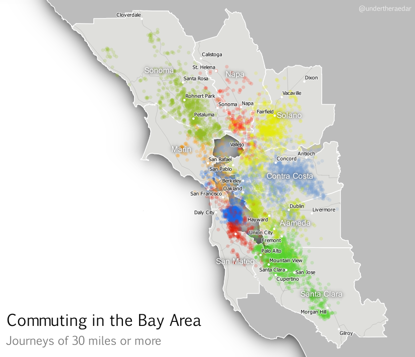
Anyway, to the point… What’s the best way of mapping polycentricity in an urban region? For this, I decided to look at the San Francisco Bay Area since it has been the subject of a few studies by one of my favourite scholars, Prof Robert Cervero of UC Berkeley. Also, a paper by Melanie Rapino and Alison Fields of the US Census Bureau identified the Bay Area as the region with the highest percentage of ‘mega commuting’ in the United States (traveling 90 or more minutes and 50 or more miles to work). Therefore, I decided to look at commuting flows between census tracts in the 9 counties of the Bay Area, from Sonoma County in the north to Santa Clara County in the south. I’ve used a cut-off of 30 miles here instead of the more generous 50 mile cut-off used by Rapino and Fields. I also mapped the whole of the United States in this way, but that’s for another day.

The series of maps below illustrate both patterns of commuting in the Bay Area and the different approaches I’ve taken in an attempt to capture the essence of polycentrism in the area. I don’t attempt to capture the misery of some of these commutes, since for that I’d need a different kind of technology. But, I do think the animations in particular capture the polycentric nature of commuter flows. If you’re represented by one of the dots in the images below, thanks a lot for taking part!

Let’s start with a simple representation of commutes of over 30 miles from San Francisco County (which is coterminous with the City of San Francisco). The animated gif is shown below and you can click the links to view the sharper video file (mp4) in your browser (so long as you're on a modern browser). The most noticeable thing here is the big blue blob© making its way down from San Francisco to Palo Alto, Mountain View and Cupertino in Santa Clara County. In total, the blue dots represent just over 15,000 commuters going to 803 different destination census tracts. I’m going to take a wild guess and suggest that some of these commutes are by people who work at Stanford, Google and Apple. But it probably also includes people working at NASA Ames Research Center, Santa Clara University and locations in San Jose. 

View video file in browser - or click image to enlarge gif

These patterns aren’t particularly surprising, since there has been a lot of press coverage about San Francisco’s bus wars and commutes of this kind. However, there is a fairly significant dispersal of San Francisco commuters north and east, even if the numbers don’t match those of the big blue blob. By the way, from San Francisco it's about 33 miles to Palo Alto, 39 miles to Mountain View, 42 to Cupertino and 48 to San Jose. 

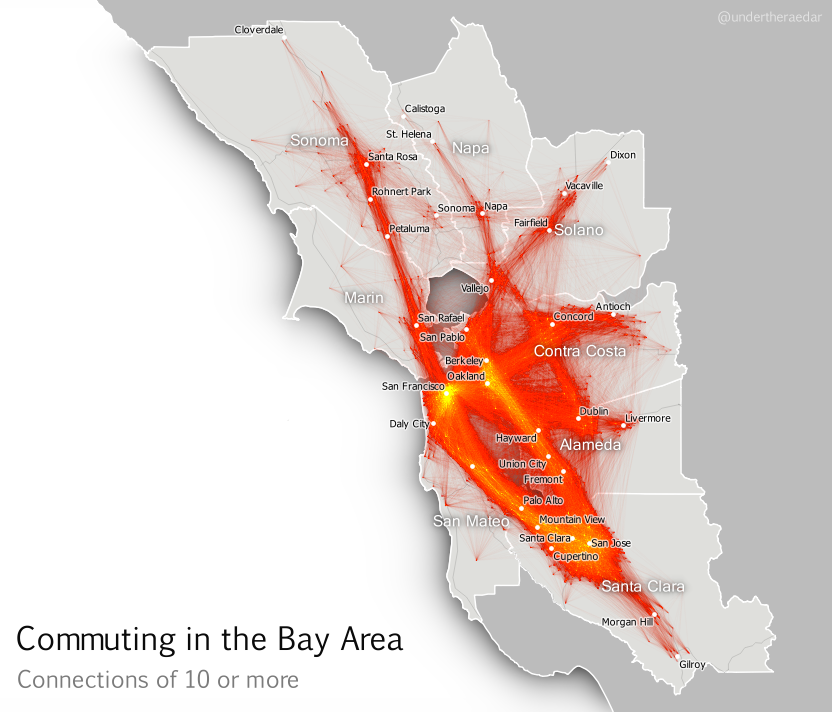
The first example above doesn’t reveal anything like the whole story, though. There are actually quite a lot of commuters who travel in the opposite direction from Santa Clara County to San Francisco but more widely the commuting patterns in the Bay Area – a metro area of around 7.5 million people – resembles a nexus of mega-commuting. This is what I’ve attempted to show below, for all tract-to-tract connections of 10 people or more, and no distance cut-off. The point is not to attempt to display all individual lines, though you can see some. I’m attempting to convey the general nature of connectivity (with the lines) and the intensity of commuting in some areas (the orange and yellow glowing areas). Even when you look at tract-to-tract connections of 50 or more, the nexus looks similar.

Click image to view larger version

Stronger connections - click image to view larger version

If we zoom in on a particular location, using a kind of ‘spider diagram’ of commuting interactions, we can see the relationships between one commuter destination and its range of origins. In the example below I’ve taken the census tract where the Googleplex is located and looked at all Bay Area Commutes which terminate there, regardless of distance. In the language of the seminal Chicago Area Transportation Study I mentioned above, these are ‘desire lines’ since this represents ‘the shortest line between origin and destination, and expresses the way a person would like to go, if such a way were available’ (CATS, 1959, p. 39) instead of, for example, sitting in traffic on US Route 101 for 90 minutes. According to the data, this example includes just over 23,000 commuters from 585 different locations across the Bay Area. I've also done an animated line version and a point version, just for comparison.

Commuting connections for the Googleplex census tract

Animated spider diagram of flows to Mountain View

Just some Googlers going to work (probably) mp4

Looking further afield now, to different parts of the Bay Area, I also produced animated dot maps of commutes of 30 miles or more for the other three most populous counties – Alameda, Contra Costa and Santa Clara. I think these examples do a good job of demonstrating the polycentric nature of commuting in this area since the points disperse far and wide to multiple centres. Note that I decided to make the dots return to their point of origin – after a slight delay – in order to highlight the fact that commuting is a two way process. The Alameda County animation represents over 12,000 commuters, going to 751 destinations, Contra Costa 25,000 and 1,351, and Santa Clara nearly 28,000 commuters and 1,561 destinations. The totals for within the Bay Area are about 3.3 million and 110,000 origin-destination links.

Alameda County commutes of 30+ miles mp4

Contra Costa County commutes of 30+ miles mp4

Santa Clara County commutes of 30+ miles mp4

Finally, I’ve attempted something which is a bit much for one map, but here it is anyway; an animated dot map of all tract-to-tract flows of 30 or more miles in the Bay Area, with dots coloured by the county of origin. Although this gets pretty crazy half way through I think the mixing of the colours does actually tell its own story of polycentric urbanism. For this final animation I’ve added a little audio into the video file as well, just for fun.

A still from the final animation - view here

What am I trying to convey with the final animation? Like I said, it's too much for a single map animation but it's kind of a metaphor for the messy chaos of Bay Area commuting (yes, let's go with that). You can make more sense of it if you watch it over a few times and use the controls to pause it. It starts well and ends well, but the bits in the middle are pretty ugly - just like the Bay Area commute, like I said.

My attempts to understand the functional nature of polycentric urbanism continue, and I attempt to borrow from pioneers like Waldo Tobler and the authors of the Chicago Area Transportation Study. This is just a little map-based experimentation in an attempt to bring the polycentric metropolis to life, for a region plagued by gruesome commutes. It’s little wonder, therefore, that a recent poll suggested Bay Area commuters were in favour of improving public transit. If you're interested in understanding more about the Bay Area's housing and transit problems, I suggest watching this Google Talk from Egon Terplan (54:44).

Notes: the data I used for this are the 2006-2010 5-year ACS tract-to-tract commuting file, published in 2013. Patterns may have changed a little since then, but I suspect they are very similar today, possibly with more congestion. There are severe data warnings associated with individual tract-to-tract flows from the ACS data but at the aggregate level they provide a good overview of local connectivity. I used QGIS to map the flows. I actually mapped the entire United States this way, but that’s going into an academic journal (I hope). I used Michael Minn’s MMQGIS extension in QGIS to produce the animation frames and then I patched them together in GIMP (gifs) and Camtasia (for the mp4s), with IrfanView doing a little bit as well (batch renaming for reversing file order). Not quite a 100% open source workflow but that’s because I just had Camtasia handy. The images are low res and only really good for screen. If you’re looking for higher resolution images, get in touch. It was Ebru Sener who gave me the idea to make the dots go back to their original location. I think this makes more sense for commuting data.

The Cartographatron: Information and images on the 'Cartographatron' used in the Chicago Area Transportation Study (1959) are shown below.

From p.39 of CATS, 1959, Vol 1

From p.98 of CATS, 1959, Vol 1

Creating an English green belt atlas

UPDATE: I've fixed the glitches in version 1 and compiled a spreadsheet with the data. See new download at the bottom of the post.

I've blogged before about green belt, and also written about the underlying data in the press. Now that the data are open, I've finally got round to finishing a little project I meant to complete ages ago. I was prompted to do this during a recent visit to my department by Prof Bob Barr, a legend in the data and GIS worlds. Bob said it would be good to know what percentage of the land area in each local authority in England was covered by green belt. I agree, so here are the results of my analysis (using 2014 green belt data) from Version 1 of my English green belt 'atlas' (actually lots of individual images to keep the file size down). Here's a snapshot of one of the maps...

Green belt land in Cheshire East

And another, this time from Birmingham. You can see that I've dimmed the background so that you can get a sense of other green belt land in the areas I've mapped.

Birmingham green belt land

Finally, a few more from around the country...

There are some glitches in the data but my initial overview suggests the numbers are pretty accurate (see exceptions below). I hope that people might find these maps useful. If you want to use any of them, be my guest.

Download all the files here (154MB): Green Belt Atlas 2014 (version 2) (186 individual map files, plus spreadsheet)

Download just the spreadsheet: percent green belt figures for each of the 186 local authorities:

Contents of the spreadsheet (download above)

Warnings: A couple of issues with version 1... 1. The West Lancashire greenbelt area extends into the sea on the green belt shapefile available from DCLG, so the figures here are incorrect (working on a fix). 2. The figure for Ashfield is clearly wrong - not sure why, so I will fix that too. 3. Some areas have extremely low values and may not actually be in the green belt - it may instead be down to the accuracy of underlying data. 4. Mole Valley currently missing, am looking into why. UPDATE: I looked again at the original Green Belt shapefile from DCLG and found that Mole Valley had the same code as Ashfield, so I fixed that and there's now a map for Mole Valley. New Forest was also assigned two different codes, so I've fixed that too. Also, in the percent figure, I've exluded the part of the West Lancashire green belt that is not on land, so this gives an accurate figure now. You can see from the image below that part of the green belt goes into the Ribble Estuary.

Technical stuff: I did this in QGIS 2.8 (open source GIS software) using the Atlas tool and a very heavy laptop, plus a bit of trickery I picked up here and there. I blogged about this before, with a little tutorial. Perhaps I should actually be using the term 'green belts', as Richard Blyth pointed out, but forgive me for this.

The beating heart of the City of London

I've had a rush of blood to the head so here I am with a second blog in two days. I'm getting some slides ready for tomorrow's Modelling World 2015 talk in London, which is all about visualising mobility (see below) so I wanted to add in a couple of new visuals on commuting in and out of London. Visualisation can often be just a lot of fancy graphics. This can be useful in itself for a number of reasons (e.g. capturing attention on an important issue, drawing attention to unusual patterns in a dataset) but since I've been working with commuting data in England and Wales I wanted to focus on flows into and out of the City of London. 

This interests me for a number of reasons, including i) commuting can play a significant role in wealth creation and it also needs to be understood in relation to how we measure GVA; ii) commuting is often very stressful and damaging to the individual - particularly long commutes - so I'm interested in the kinds of distances involved and this can be seen easily on a map; iii) commuting can often be environmentally damaging - though this isn't what I'm mapping here; iv) commuting in and around London is often about green belt hopping so I was curious to see how much commuting comes from beyond the metropolitan green belt; and v) commuting is a two-way process and affects places at both ends and in between due to travel. 

So, here's what I did. I took the MSOA-level commuting data for England and Wales (table WUEW01 here), used a bit of QGIS, extracted frames from QGIS using the MMQGIS plugin, then patched it all together in GIMP to create an animated gif. One for inflows, one for outflows and one for in and outflows (thanks to Ebru Sener for the idea). It might run a little slowly in the blog post in a browser but see below for the images. Just to clarify, I've only shown flows of 25 or more into the City of London. Those not familiar with the data should be aware the the 'City of London' refers to the small area in the centre of London and not the entirity of Greater London! An obvious point but one worth repeating in case anyone is confused. A Greater London map would have many more data points, covering most of England.

Commuting flows (>=25) into the City of London

Same as above, but going back the way

The 'pulse' of the City of London

You should be able to get a better view of the images by clicking on them individually and if you want them to work more quickly try saving them to your own machine.